Epoch 7: Makemore, Part 4
Intro
Hi, I’m Mon, in the previous epoch we learnt how to make the backward pass of the bigram and make a one layer neural net, which the result of the training would be approximately equal to “normalizing the counts” approach, then we began to build mlp and context of 3 chars to predict the 4th chars. We continue to build the mlp of Makemore in this epoch.
Content: MLP Part 3
We have already created the second layer of the mlp with tanh:
h = torch.tanh(emb.view(-1, 6) @ W1 + b1)
Now we need to create the third (last layer)
W2 = torch.randn(100,27)
b2 = torch.randn(27)
logits = h @ W2 + b2

logits.shape
#torch.Size([32, 27])
and
counts = logits.exp()
prob = counts / counts.sum(1, keepdims =True)
prob[torch.arange(32), Y]
This shows the probability of feeding with the context index and getting the 4th letter.
Now at last we calculate the loss:
loss = -prob[torch.arange(32), Y].log().mean()

loss
#tensor(15.9918)
We need to minimize this number…
to understand the reason why we used neg log mean, read the previous epoches.
Summary
#init

g = torch.Generator().manual_seed(367452352)
C = torch.randn((27, 2), generator=g)
W1 = torch.randn((6, 100), generator=g)
b1 = torch.randn((100), generator=g)

W2 = torch.randn((100, 27), generator=g)
b2 = torch.randn((27), generator=g)

parameters = [C, W1, b1, W2, b2]
for p in parameters:
    p.requires_grad = True

sum(p.nelement() for p in parameters)
#3481
nelement() counts the elements of a matrix
#forward pass

emb = C[X]
h = torch.tanh(emb.view(-1, 6) @ W1 + b1)
logits = h @ W2 + b2
counts = logits.exp()
prob = counts / counts.sum(1, keepdims=True)
loss = -prob[torch.arange(32), Y].log().mean()
loss
#tensor(15.9918)
Note:In the bigram, we used one-hot encoding to convert indices into numerical vectors, and then multiplied them by W. This multiplication effectively selects one row of W, because each one-hot vector contains a single 1.
In the MLP model, Instead of one-hot vectors, we directly index into the embedding matrix using C[X], which chooses the corresponding rows of C. This is more efficient and mathematically equivalent to one-hot encoding followed by a matrix multiplication.
cross_entropy
Instead of calulating counts, probs, and loss(neg log mean), for efficiency we can use cross_entropy to let pytorch compute logits to loss!
logits(raw score) -> loss
emb = C[X]
h = torch.tanh(emb.view(-1, 6) @ W1 + b1)
logits = h @ W2 + b2
# counts = logits.exp()
# prob = counts / counts.sum(1, keepdims=True)
# loss = -prob[torch.arange(32), Y].log().mean()
loss = F.cross_entropy(logits, Y)
Let's make our autograd:
for _ in range(10):
    #forward pass
    emb = C[X]
    h = torch.tanh(emb.view(-1, 6) @ W1 + b1)
    logits = h @ W2 + b2
    # counts = logits.exp()
    # prob = counts / counts.sum(1, keepdims=True)
    # loss = -prob[torch.arange(32), Y].log().mean()
    loss = F.cross_entropy(logits, Y)
    print(loss.item())


    #backward pass
    for p in parameters:
        p.grad = None

    loss.backward()

    #update
    for p in parameters:
        p.data += -0.1 * p.grad
the result of the loss after many trainings, is around, 0.25
The reason is because some contexts (’. . .’) have different 4th chars. So the autograd cannot determine one specific 4th letter for all specific contexts such as
‘. . .’ context.
Mini Batch
Now that we want to use all the names/words, there are 228146 contexts, and it is more efficient to use mini batches instead.
By randomly select random portion of dataset, and only do forward pass, backward pass, and updates those mini batches.
ix = torch.randint(0, X.shape[0], (32,))
This creates 32 random ints, between 0 and the X.shape[0] which is 228146.
Now our new autograd is:
for _ in range(10):
    ix = torch.randint(0, X.shape[0], (32,))

    #forward pass
    emb = C[X[ix]] #changed


    h = torch.tanh(emb.view(-1, 6) @ W1 + b1)
    logits = h @ W2 + b2
    # counts = logits.exp()
    # prob = counts / counts.sum(1, keepdims=True)
    # loss = -prob[torch.arange(32), Y].log().mean()
    loss = F.cross_entropy(logits, Y[ix]) #changed


    print(loss.item())

    #backward pass
    for p in parameters:
        p.grad = None

    loss.backward()

    #update
    for p in parameters:
        p.data += -0.1 * p.grad
Note: The quality of gradient is lower, but the gradient direction is still a good approximation if we do it in small size with more steps.
Determining the right update size of W
To do so we need to create a plot, update W with different step sizes, and compare the loss on the plot.
lre = torch.linspace(0.001, 1, 1000)
This creates 1000 steps, between 0.001 to 1
e.g.
[0.0010, 0.0020, 0.0030,...
But let’s use torch.logspace(-3, 0, 1000),
This creates 1000 steps, between 10^-3 to 10^0
Simply because learning rate effects are multiplicative, not additive
outside the loop:
logsi = torch.logspace(-3, 0, 1000)
lrs = []
allloss = []
inside forward pass:
lr = logsi[i]
allloss.append(loss.item())
after all:
lrs.append(lr)
full code:
logs = torch.logspace(-3, 0, 1000)
lrs = []
allloss = []

for i in range(1000):
    ix = torch.randint(0, X.shape[0], (32,))

    #forward pass
    lr = logs[i]
    emb = C[X[ix]]
    h = torch.tanh(emb.view(-1, 6) @ W1 + b1)
    logits = h @ W2 + b2
    # counts = logits.exp()
    # prob = counts / counts.sum(1, keepdims=True)
    # loss = -prob[torch.arange(32), Y].log().mean()
    loss = F.cross_entropy(logits, Y[ix])
    print(loss.item())
    allloss.append(loss.item())


    #backward pass
    for p in parameters:
        p.grad = None

    loss.backward()

    #update
    for p in parameters:
        p.data += -lr * p.grad

    lrs.append(lr)
Now the plot:
plt.plot(lrs,allloss)
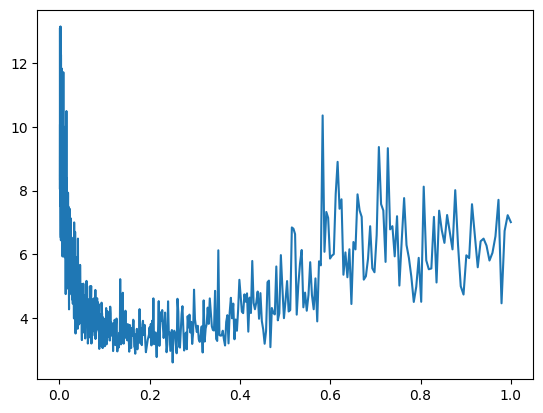
x: lrs, y: allloss
As you see the best learning rate is in the area of 0.1 and 0.2
So let’s choose 0.1 and run many steps, to get more precise result, after many steps, we use 10x lower step size: 0.01 and then run the code and check the loss, and then continue the training…
split dataset into 3 splits
We split our dataset into 3 splits:
Training, validation, and test splits
Learning the weights: by gradient descent (training set) 80% of our dataset
Choosing hyperparameters: by observing results (validation set), we compare the model sizes, learning rates, embedding size, strength of regularization and decide when to stop the training,
Note: no backward() in this set at all
Final performance: by unbiased and untouched test set
Note: We are only allowed to check loss in test set only a few times, to prevent overfitting and bias of tester.
Now let’s make our new autograd with these splits:
#init
block_size = 3
def build_dataset(words):
  X, Y = [], []
  for w in words:

    context = [0] * block_size
    for ch in w + '.':
      ix = stoi[ch]
      X.append(context)
      Y.append(ix)
      context = context[1:] + [ix] # sliding window

  X = torch.tensor(X)
  Y = torch.tensor(Y)
  print(X.shape, Y.shape)
  return X, Y

import random
random.seed(42)
random.shuffle(words)
n1 = int(0.8*len(words))
n2 = int(0.9*len(words))

Xtr, Ytr = build_dataset(words[:n1])
Xdev, Ydev = build_dataset(words[n1:n2])
Xte, Yte = build_dataset(words[n2:])
First we shuffle or randomize the words.
We can feed this function with n1(80%) to achieve the trainingg set(Xtr, Ytr), or from n1 80% to n2 90% = 10% for the dev set (Xdev, Ydev) or the rest of the n2 90% to 100% = 10% for the test set (Xte, Yte)
Same parameters(we can change the neuron counts)
g = torch.Generator().manual_seed(2147483647)
C = torch.randn((27, 10), generator=g)
W1 = torch.randn((30, 200), generator=g)
b1 = torch.randn(200, generator=g)
W2 = torch.randn((200, 27), generator=g)
b2 = torch.randn(27, generator=g)
parameters = [C, W1, b1, W2, b2]
for i in range(1000):
    ix = torch.randint(0, Xtr.shape[0], (32,))

    #forward pass
    #lr = logs[i]
    emb = C[Xtr[ix]]
    h = torch.tanh(emb.view(-1, 6) @ W1 + b1)
    logits = h @ W2 + b2
    # counts = logits.exp()
    # prob = counts / counts.sum(1, keepdims=True)
    # loss = -prob[torch.arange(32), Y].log().mean()
    loss = F.cross_entropy(logits, Ytr[ix])
    # print(loss.item())
    # allloss.append(loss.item())


    #backward pass
    for p in parameters:
        p.grad = None

    loss.backward()

    #update
    for p in parameters:
    #   p.data += -lr * p.grad
        p.data += -0.01 * p.grad

    # lrs.append(lr)
print(loss.item())
As you may noticed we just changed the X with Xtr and Y with Ytr. To calcualte the X and Y of dev and test sets, we can put these outside the loop:
# validation loss
emb = C[Xdev] # (32, 3, 10)
h = torch.tanh(emb.view(-1, 6) @ W1 + b1) # (32, 100)
logits = h @ W2 + b2 # (32, 27)
loss = F.cross_entropy(logits, Ydev)
loss

# test loss
emb = C[Xte] # (32, 3, 10) emb dim C = 10
h = torch.tanh(emb.view(-1, 6) @ W1 + b1) # (32, 100)
logits = h @ W2 + b2 # (32, 27)
loss = F.cross_entropy(logits, Yte)
loss
Note: we are printing the validation and test loss outside the loop of training set.
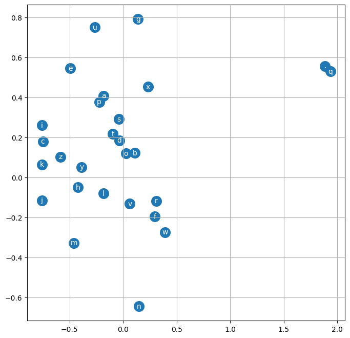
plot C
Since our C embedded dim is 2 for each char, we can consideer each as an axis, and plot the char with that 2 dims.
# visualize dimensions 0 and 1 of the embedding matrix C for all characters
plt.figure(figsize=(8,8))
plt.scatter(C[:,0].data, C[:,1].data, s=200)
for i in range(C.shape[0]):
    plt.text(C[i,0].item(), C[i,1].item(), itos[i], ha="center", va="center", color='white')
plt.grid('minor')
plotting parameters, shows valuable data such as: Inputs that are near each other have similar likelihood of occurrence, the closer they are, the more interchangeable they are.
Sampling
After we trained our model, let’s pick some names as samples:
g = torch.Generator().manual_seed(2147483647 + 10)

for _ in range(20):

    out = []
    context = [0] * block_size
    while True:
      emb = C[torch.tensor([context])]
      h = torch.tanh(emb.view(1, -1) @ W1 + b1)
      logits = h @ W2 + b2
      probs = F.softmax(logits, dim=1)
      ix = torch.multinomial(probs, num_samples=1, generator=g).item()
      context = context[1:] + [ix]
      out.append(ix)
      if ix == 0:
        break

    print(''.join(itos[i] for i in out))