Epoch 6: Makemore, Part 3
Intro
Hi, I’m Mon, in the previous epoch we learnt how to create the forward pass, we need to create our backward pass too
Content: Bigram Part 8: Make forward pass for bigrams
At first lets learn some definitions:
in Classification we predict a label such as cat vs dog.
in Regression we predict a number or value.
In each of these we use different approaches to calculate the loss
in our micrograd we used mean squared error, and here we use neg log probs
From the previous epoch the forward pass
Step 1: init g and W
g = torch.Generator().manual_seed(145324423)
W = torch.randn((28, 28), generator=g)
Step 2: forward pass:
xenc = F.one_hot(xs, num_classes=28).float()
logits = xenc @ W
counts = logits.exp()
probs = counts / counts.sum(1, keepdims=True)
loss
Instead of the loop (check the end of epoch 5), let's make the loss computation more straightforward
we can use a better vectorized method:
loss = -probs[torch.arange(5), ys].log().mean()
torch.arange(n,m) simply creates a vector with items n to m in order.
Content: Bigram Part 9: Make backward pass for bigrams
Step 3: set gradient of W to 0
W.grad = None
Step 4: backward()
loss.backward()
W.grad.shape
#torch.Size([28, 28])
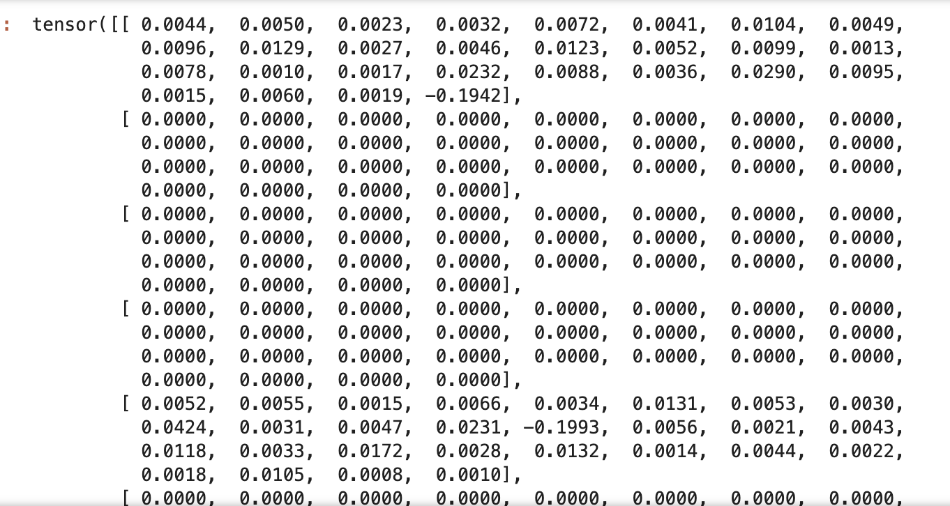
At this point we stored the gradients of W, check:
W.grad
Step 5: update Weights
W.data += -0.1 * W.grad
We can repeat the process of forward -> check loss -> backward and store the new gradients of W -> update W -> forward and repeat
xenc = F.one_hot(xs, num_classes=28).float()
logits = xenc @ W
counts = logits.exp()
probs = counts / counts.sum(1, keepdims=True)
loss = -probs[torch.arange(5), ys].log().mean()
loss.item()
W.grad = None
loss.backward()
W.data += -0.01 * W.grad
Until now we used one word, and did the forward backward, and training steps manually, let’s make a loop that does the autograd many times and for all the dataset of the names,
#init
xs, ys = [], []
for w in words:
    chars = ['<S>'] + list(w) + ['<E>']
    for char1, char2 in zip(chars, chars[1:]):
        ix1 = stoi[char1]
        ix2 = stoi[char2]
        xs.append(ix1)
        ys.append(ix2)
xs = torch.tensor(xs)
ys = torch.tensor(ys)
num = xs.nelement()

g = torch.Generator().manual_seed(145324423)
W = torch.randn((28, 28), generator=g, requires_grad=True)
#gradient descent
for k in range(100):
    #forward pass
    xenc = F.one_hot(xs, num_classes=28).float()
    logits = xenc @ W
    counts = logits.exp()
    probs = counts / counts.sum(1, keepdims=True)
    loss = -probs[torch.arange(num), ys].log().mean()
    print(loss.item())

    #backward
    W.grad = None
    loss.backward()

    #update
    W.data += -10 * W.grad

#3.8504281044006348
#3.755488872528076
#3.6703531742095947
#3.593259334564209
#3.5231285095214844
#3.4592230319976807
#3.400963306427002
#3.347846508026123
#3.299407482147217
#3.2552058696746826
#3.2148220539093018
.
.
.
#2.575495481491089
The optimized loss will be around 2.5, which is the same when we calculate with the number of occurrences:
n = 0
sumlogprobs = 0.0

for w in words:
#for w in ["monqf"]:
    chs = ['<S>'] + list(w) + ['<E>']
    for ch1, ch2 in zip(chs, chs[1:]):
        ix1 = stoi[ch1]
        ix2 = stoi[ch2]
        prob = dist_all[ix1, ix2]
        logprob = torch.log(prob)
        n += 1

        neglogprob = -logprob
        sumlogprobs += neglogprob
       # print(f'{ch1}, {ch2}: {prob:.3f} {logprob: .4f} {neglogprob: .4f}')


print(n)
print(sumlogprobs)
print((sumlogprobs/n).item())

#228146
#tensor(559962.3125)
#2.4544034004211426
As you see, roughly, we are getting the same result with the counting and normalizing method because we are using a simple linear one layer, but later we will add more complexities, neurons and non-linearity, increase contexts(not just 2 characters bigrams) to create a better nn and lower the loss.
Note: For smoothing our dataset to prevent extremes, including infinity, we added a small number to the items of our dataset,
There is another way for smoothing called
regularization loss: a penalty added to the loss that discourages extreme or overly confident weights in W.
e.g. Making W closer to 0, can make the loss more unified, so
loss = -probs[torch.arange(num), ys].log().mean() + 0.01*(W**2).mean()
Content: Bigram Part 10: sampling
Now let’s pick some names as the sampling of our nn model by generating names.
#sampling
g = torch.Generator().manual_seed(145324423)

for i in range(5):

    name = []
    ix = 0
    while True:
        xenc = F.one_hot(torch.tensor([ix]), num_classes=28).float()
        logits = xenc @ W
        counts = logits.exp()
        probs = counts / counts.sum(1, keepdims=True)

        ix = torch.multinomial(probs, num_samples=1, replacement=True, generator=g).item()
        name.append(itos[ix])
        if ix == 27:
            break
    print(''.join(name))
melylin
<E>
tosh<E>
elinen<E>
n<E>
gsahrmaquan<E>
You can access the code here: https://github.com/auroramonet/memo/blob/main/codes/makemore1.ipynb
Content: MLP Part 1
Now we are getting into making a multi layer neural net,
Karpathy introduced Bengio et al. 2003 (MLP language model) paper.
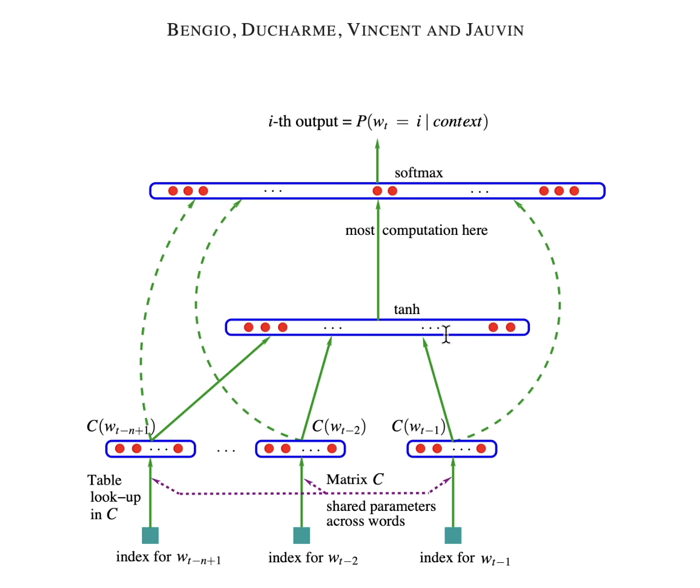
The paper shows the structure of building a language model, which has 18k words,
feed 3 words and predict the 4th word.
At the bottom, we have 3 words, which they have an index in the 17k words dataset.
Then each of these words use look up table C(matrix of 17k * num of neurons or embedding dim (e.g. 30)) which corresponds to the embedding vector for that word.
for each word:
row: 17k
column: 30
in here the input layer has 3 words * 30 neurons = 90 neurons
In the hidden layer, we can use any size (hyper parameter), and all of the neurons are fully connected to the previous layer of neurons (90)
In the output layer, we have 17k neurons (all words), all are connected to the hidden layer, 17k logits -> softmax -> prob. dist. –> L , then sampling the 4th word index (or in training phase: fine tuning the parameters to minimize the loss for the correct 4th word)
all parameters: weights and biases of all layers
We are going to make our 3+1 chars dataset, input 3 words, output 4th words (compare with the previous bigrams input 1, output 1)
Let’s begin with making our chars, stoi and itos:
import torch
import torch.nn.functional as F
import matplotlib.pyplot as plt
%matplotlib inline

words = open('names.txt', 'r').read().splitlines()
chars = sorted(list(set(''.join(words))))
stoi = {s:i+1 for i,s in enumerate(chars)}
stoi['.'] = 0
itos = {i:s for s,i in stoi.items()}
print(itos)

#{1: 'a', 2: 'b', 3: 'c', 4: 'd', 5: 'e', 6: 'f', 7: 'g', 8: 'h', 9: 'i', 10: 'j', 11: 'k', 12: 'l', 13: 'm', 14: 'n', 15: 'o', 16: 'p', 17: 'q', 18: 'r', 19: 's', 20: 't', 21: 'u', 22: 'v', 23: 'w', 24: 'x', 25: 'y', 26: 'z', 0: '.'}
Now let’s begin with making dataset of 3 words -> 4th word
#dataset
block_size = 3 #L1
X, Y = [], [] #L2
for w in words[:5]: #L3

    print(w)
    context = [0] * block_size #L6
    for ch in w + '.': #L7
        ix = stoi[ch] #L8
        X.append(context)
        Y.append(ix)
        print(''.join(itos[i] for i in context), '--->', itos[ix])
        context = context[1:] + [ix] #L12


X = torch.tensor(X)
Y = torch.tensor(Y)
Line 1: Block size is the context length (how many items in each context)
Line 2: X is context(inputs)
Y is the label (outputs, or in here the 4th char)
Line 6: Init 1st row of context with [0,0,0]
Line 7: We add ‘.’ to the end of each name, and use the items of a name (characters) in the loop
in our example the first name is emma, so the first char is ’e’
Note: in here context is cleared after each loop, but we store each context in X,
until now we have [0,0,0] in the context, and we append it to the X
and we append the char, here ’e’ to Y, so the first element of Y is ’e’
We created our first X and first Y
Line 12: Sliding Window to create the next context: We omit the oldest char and add the next char ix
Now our new context is [0,0,5], which in the next loop will be added as the next row of X
X will be something like:
[0,0,0],
[0,0,5],
and Y will be like:
[5,13]
Content: MLP Part 2
Now let’s create the lookup table C with starting embedding dimension of 2 for each word
C = torch.randn((27, 2))
We can look up index of a tensor e.g.:
C[3]
#tensor([0.8668, 0.2768])
and also we can look up more than one rows. e.g.
C[[3,2,2,2,1]]
#tensor([[ 0.8668,  0.2768],
        [-0.0414, -1.0714],
        [-0.0414, -1.0714],
        [-0.0414, -1.0714],
        [ 0.5640, -0.1473]])
Embedding Lookup:
C[X]: We are gathering rows from C according to indices in X
C.shape = (a, b)
X.shape = (x, y)
C[X].shape (x,y,b)
This means x tables of [y,b] size
Example:
# C.shape: (27, 2)
# X.shape: (3,3)

X =
[
  [0, 0, 1],
  [0, 1, 2],
  [0, 0, 1],
]


C[X] =
[
  [C[0], C[0], C[1]],
  [C[0], C[1], C[2]],
  [C[0], C[0], C[1]],
]
C[X][1]
#[C[0], C[0], C[1]]

C[X][1,2]
#C[1]

C[X][1,2,0]
#the first item of C[1]
Note: You can see the column of C as the dimension of input X, which it means each input X now has “column of C” times dimension.
Let’s call C[X]: emb
emb = C[X]
emb.shape

#torch.Size([32, 3, 2])
#2: dim
Init W and b:
W1 = torch.randn((6, 100))
b1 = torch.randn(100)
Now we need to multiply our emb with the weights and add bias like:
emb @ W1 + b1
But this is not working, because of the matrix multiplication rule:
In (A @ B)
The last dimension of A must be equal with the first dimension of B
So in here since the shape of W1 is (6,100) and the first dim is 6, the last dim of emb must be 6 to be able to do the multiplication of the matrix.
So let’s convert [32, 3, 2] -> [32, 6]
To do so, we decompose the shape into 3 parts of [32, 2] then concatenate them with cat to achieve [32,6]
torch.cat([emb[:, 0, :]],[emb[:, 1, :]],[emb[:, 2, :]], 1).shape

#torch.Size([32, 6])
cat rule 1: All tensors must have the same shape in every dimension except dim
e.g. in here dim=1
Another better way to do so is using unbind:
torch.unbind(emb, 1)
This removes a tensor dim glues and convert it to lists of tensors, in here it cut the glues of dim 1
now to glue them in dim 1 we use:
torch.cat(torch.unbind(emb, 1), 1)
.view()
We can change the dimension view of a matrix simply if the multiplication of their dims are equal, e.g.
m = torch.arange(18)
m
#tensor([0,1,2,3,4,5,6 ... 17])
m.shape
#torch.Size([18]) 1 dim

m.view(3, 3, 2)

tensor([[[ 0,  1],
         [ 2,  3],
         [ 4,  5]],

        [[ 6,  7],
         [ 8,  9],
         [10, 11]],

        [[12, 13],
         [14, 15],
         [16, 17]]])
m.view(9, 2)
tensor([[ 0,  1],
        [ 2,  3],
        [ 4,  5],
        [ 6,  7],
        [ 8,  9],
        [10, 11],
        [12, 13],
        [14, 15],
        [16, 17]])
The reason for this is because in the memory, the items of a tensor, regardless of the dims, are stored flat, 1 dim, e.g:
m.storage()
0
 1
 2
 3
 4
 5
 6
 7
 8
 9
 10
 11
 12
 13
 14
 15
 16
 17
[torch.storage.TypedStorage(dtype=torch.int64, device=cpu) of size 18]
So instead of unbinding and concatenating, we can use the view directly, because it is so efficient and simple
emb.view(32, 6)

#verify
emb.view(32, 6) == torch.cat(torch.unbind(emb, 1), 1)
#tensor([[True, True, True, True, True, True],
# [True, True, True, True ,...
Now that we know this method works, let's do:
h = emb.view(32, 6) @ W1 + b1
h.shape

#torch.Size([32, 100])
# instead of 32 we can use
# emb.shape(0)
# or
# -1
Note: when saying -1, pytorch automatically and internally calcualtes the total number of elements, and since we gave the other dims sizes, it will calcualte the first dim size
Adding tanh
h = torch.tanh(emb.view(-1, 6) @ W1 + b1)