Epoch 5: Makemore, Part 2
Intro
Hi, I’m Mon, this is Epoch 5, Makemore p2
Content: Bigram Part 4: Better efficiency
Just a concept to know, before we begin:
Broadcasting:
Broadcasting is when PyTorch automatically “stretches” a smaller tensor to match a larger one so element-wise operations can work without copying data.
e.g.
A = torch.tensor([[1, 2, 3], [4, 5, 6]])
# A.shape: (2, 3)

b = torch.tensor([10, 20, 30])
# b.shape: (3,)
A + b
e.g. in here it streches (reuse, not duplicate) [10, 20, 30] internally
Rule 1: Dimension sizes must be equal, one of them is “1” or one of them does not exist.
Rule 2: For streching the smaller vector, bring them to the right (right-aligned)
e.g. [27,27,27] + [27,27]
[27,27] -> [ ,27,27] -> [1,27,27] -> [27,27,27]
As you may noticed in this part:
dist_all = N[ix].float()
dist_all /= dist_all.sum()
For every character of a name, we calculate the prob. dist. every time which is inefficient. Now we decide to compute prob. dist. at once, for the whole tensor
Before we begin to implement that, we need to know some concepts.
Let me compare 2 approaches to find the more efficient way
approach 1:
dist_all = N[ix].float()
dist_all /= dist_all.sum()
1.1. N[ix].shape: (28,) 1D
1.2. Not vectorized
1.3. Loops 1 row at a time, poor scaling
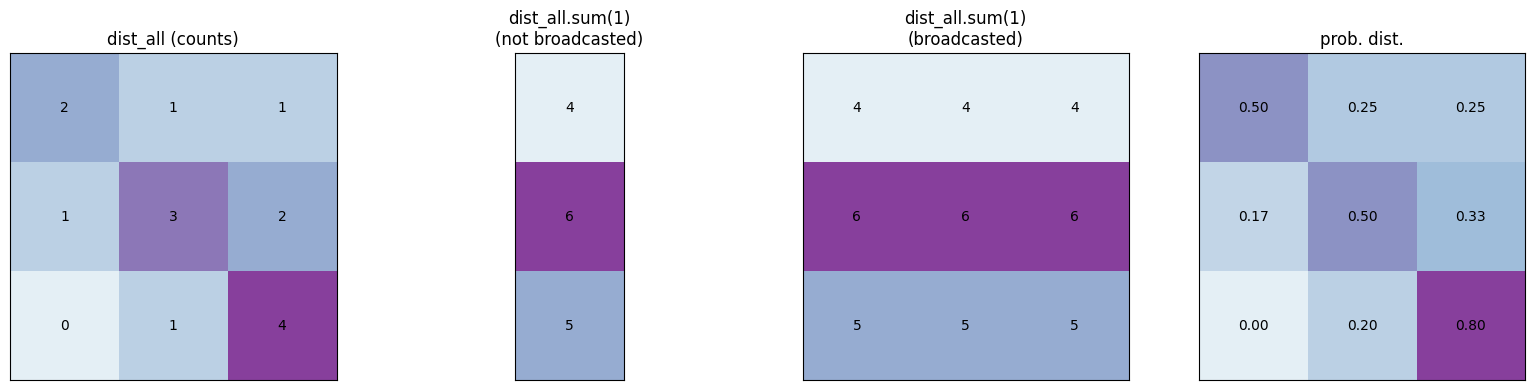
approach 2:
dist_all = N.float()
dist_all /= dist_all.sum(1)
2.1: firstly: N.shape: (28,28)
2.2: secondly: dist_all.sum(1)
Basically, sum(1)
means sum of all columns
row1 = column a1 + column a2 + column a3 + …
row2 = column b1 + column b2 + column b3 + …
…
sum(0) means sum of all rows
column1 = row a1 + row a2 + …
column2 = row b1 + b2 + …
Note The product of dist_all.sum(0) or dist_all.sum(1) will be a 1D tensor vector n (no row or column)
(n,)
not having 2D can be problematic, because of Broadcasting, so we need to explicitly store the dimension in the result, simply by adding keepdim=True,
so dist_all.sum(1, keepdim=True)
Gives us a 2D vector: (28, 1)
and dist_all.sum(0, keepdim=True)
Gives us a 2D vector: (1, 28)
2.3: thirdly:
dist_all /= dist_all.sum(1)
correctly boradcasts the 1D vector (28, 1) to (28, 28),
now each row of dist_all.sum(1) has 28 repeated number which is calculated previously,
then each value in our tensor (dist_all) is divided by the corresponding dist_all.sum(1)
-> The new name gen with better efficiency:
dist_all = N.float()
dist_all /= dist_all.sum(1, keepdim=True)
g = torch.Generator().manual_seed(11224234)

for n in range(10):
    out = []
    ix = 0
    while True:
        ix = torch.multinomial(dist_all[ix], num_samples= 1, replacement=True, generator=g ).item()
        out.append(itos[ix])
        if ix == 27:
            break
    print(''.join(out))
Content: Bigram Part 5: Quantized quality of a model
In the previous step, we made the prob. dist. calculator, and sampling with the prob. dist.
in the upcoming steps we are going to make nn model
Before that, we need to create a loss function, a quantifier that shows the quality of our model when we change the parameters (in here: characters)
Let’s begin with this:
dist_all = N.float()
dist_all /= dist_all.sum(1, keepdim=True)

for w in words[:3]:
    chs = ['<S>'] + list(w) + ['<E>']
    for ch1, ch2 in zip(chs, chs[1:]):
        ix1 = stoi[ch1]
        ix2 = stoi[ch2]
        prob = dist_all[ix1, ix2]
        print(f'{ch1}, {ch2}: {prob:.3f}')

#<S>, e: 0.048
#e, m: 0.038
#m, m: 0.025
#m, a: 0.390
#a, <E>: 0.196
#<S>, o: 0.012
#o, l: 0.078
#l, i: 0.178
#i, v: 0.015
#v, i: 0.354
#i, a: 0.138
#a, <E>: 0.196
#<S>, a: 0.138
#a, v: 0.025
#v, a: 0.250
#a, <E>: 0.196
- This simply shows the probability of the occurrences of the word 2 following the word 1, among the set of the word1-word2s, closer to 1 means higher likelihood to happen
-> Let’s convert these small numbers into larger indicators for convenience of calculation:
Similar to loss function in micrograd, we want to use positive number, approaching to 0
Let's do neg log:
$-\log(\text{prob})$ from 0 to 1
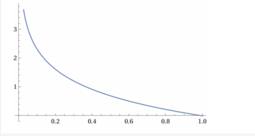
This is aligned well with the requirements:
1. lower probability (0): higher loss
2. higher probabilty (1): 0 loss
for w in words[:3]:
    chs = ['<S>'] + list(w) + ['<E>']
    for ch1, ch2 in zip(chs, chs[1:]):
        ix1 = stoi[ch1]
        ix2 = stoi[ch2]
        prob = dist_all[ix1, ix2]
        logprob = torch.log(prob)
        neglogprob = -logprob
        print(f'{ch1}, {ch2}: {prob:.3f} {logprob: .4f} {neglogprob: .4f}')

#<S>, e: 0.048 -3.0408  3.0408
#e, m: 0.038 -3.2793  3.2793
#m, m: 0.025 -3.6772  3.6772
#m, a: 0.390 -0.9418  0.9418
#a, <E>: 0.196 -1.6299  1.6299
#<S>, o: 0.012 -4.3982  4.3982
#o, l: 0.078 -2.5508  2.5508
#l, i: 0.178 -1.7278  1.7278
#i, v: 0.015 -4.1867  4.1867
#v, i: 0.354 -1.0383  1.0383
#i, a: 0.138 -1.9796  1.9796
#a, <E>: 0.196 -1.6299  1.6299
#<S>, a: 0.138 -1.9829  1.9829
#a, v: 0.025 -3.7045  3.7045
#v, a: 0.250 -1.3882  1.3882
#a, <E>: 0.196 -1.6299  1.6299
Now that we know the prob. of occurrence of bigrams, we can calculate the prob. of occurrence of a name, with multiplication of prob. of bigrams
$$ P(\text{name}) = P(e \mid \langle S \rangle) \cdot P(m \mid e) \cdot P(m \mid m) \cdot P(a \mid m) \cdot P(\langle E \rangle \mid a) $$
prob(name) = prob(bigram1) * prob(bigram2) * ...
And since we are using log, this rule applies:
$$ \log(a \cdot b \cdot c \cdot \ldots) = \log(a) + \log(b) + \log(c) + \ldots $$
Simply by defining n = 0 and sumlogprobs = 0 outside the loop and using them inside the inner loop:
     sumlogprobs += neglogprob
     n += 1
then if I print:
print(sumlogprobs)
print((sumlogprobs/n).item())

#tensor(38.7856)
#2.424102306365967
2.4241023 considered as our loss function (quality of our model)
note: We normalize the neg of log with average , it’s just better fairer since names can get long or short.
Now let’s try to see the possibility of showing up bigrams of a name and loss of a name w.r.t model parameters (bigram prob. dist.)
for w in ["mon"]:
     #same code
     .
     .
     .
#<S>, m: 0.079 -2.5354  2.5354
#m, o: 0.068 -2.6875  2.6875
#o, n: 0.304 -1.1911  1.1911
#n, <E>: 0.369 -0.9969  0.9969
#4
#tensor(7.4109)
#1.8527252674102783
Content: Bigram Part 6: Model Smoothing
If we try with a rare name which has a bigram of 0% occurrence w.r.t model parameters (bigram prob. dist.),
because we are using logarithm, at point 0, the value goes to infinity, and it causes error in our loss calculation.
e.g.
for w in ["monqf"]:
     #same code
     .
     .
     .
#<S>, m: 0.079 -2.5354  2.5354
#m, o: 0.068 -2.6875  2.6875
#o, n: 0.304 -1.1911  1.1911
#n, q: 0.000 -9.1230  9.1230
#q, f: 0.000 -inf  inf
#f, <E>: 0.088 -2.4259  2.4259
#6
#tensor(inf)
#inf
As you see the prob. of the bigram “q, f” is zero.
Solution: Using Model Smoothing, by adding a small number to our dataset (e.g. 1)
dist_all = (N+1).float()
If we add a large amount, the bigram prob. will be more similar and unified.
Content: Bigram Part 7: Make forwardpass for bigrams
Until here we could make a character level language model, sampling new names w.r.t model parameters (bigram prob. dist.), and evaluating the quality of the model neg log.
But we need to make it learnable with neural network, and tune the parameters by evaluating the loss
Step 1: Create training set of all bigrams
If you remember from the micrograd, in a neural network, we need to have inputs and outputs. In here inputs are first characters(n), and putputs are second characters in bigrams(n+1).
We feed the nn with a character, and expect to receive the correct output.
Let’s make the set of inputs and outputs
xs, ys = [],[]

for w in words[1]:
    chs = ['<S>'] + list(w) + ['<E>']
    for ch1, ch2 in zip(chs, chs[1:]):
        ix1 = stoi[ch1]
        ix2 = stoi[ch2]
        xs.append(ix1)
        ys.append(ix2)

xs = torch.tensor(xs)
ys = torch.tensor(ys)

xs
tensor([26,  4, 12, 12,  0])

ys
tensor([ 4, 12, 12,  0, 27])
Loop over all characters
Append all characters x in xs, and append all x+1 characters to ys
So bigram 1: xs[0] and ys [0]: 26,4
But there is an issue here, we have the index of the charaters (integers), they are like labels, but we need numerical values for the charcters that we can do math on them in nn. This is where we use One-hot encoding
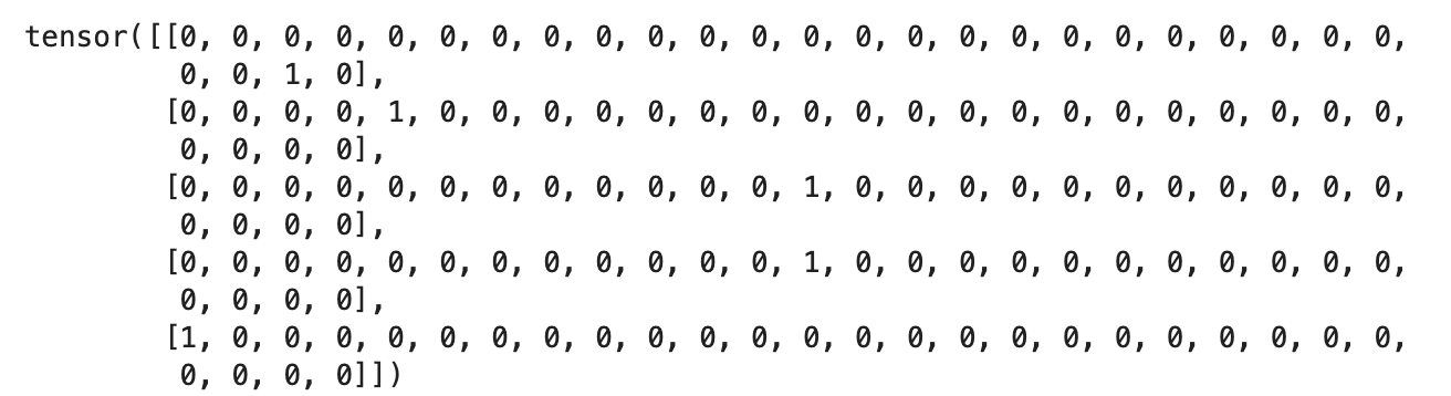
One-hot encoding: Represents a character by a vector with a single 1 at its index and zeros everywhere else.
e.g
import torch.nn.functional as F
xenc = F.one_hot(xs, num_classes=28).float()
xenc.shape
#torch.Size([5, 28])
xenc
plt.imshow(xenc)
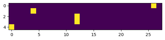
Note one_hot doesnt support .. dtype=torch.float32, instead we use .float()
Let’s make the other part of nn, initializing weights with random numbers
W = torch.randn(28, 1)
neuron = xenc @ W [3, 13]

#tensor([[-0.1169],
#        [ 0.8696],
#        [ 1.4481],
#        [ 1.4481],
#        [ 0.4780]])
W = torch.randn(28, 1) means 28 inputs and 1 output neuron.
And also each row shows the numbers related to a specific input for all neurons, and each column shows all the weights of one neuron for different inputs.
@ is matrix multiplication in line 2, we are basically multiplying xenc [n, 28] here [5,28] with [28,1]
Product Shape is [5,1] Based on the Matrix multiplication shape rule:
$$ \text{shape}(A) = (m, n), \quad \text{shape}(B) = (n, p), \quad A @ B \rightarrow \text{shape}(m, p) $$
note: torch.rand returns a tensor with a random number from the standard normal distribution
By doing the matrix multiplication we feed each neuron with n inputs
We can increase the number of the neurons too:
W = torch.randn(28, 28)
neurons = xenc @ W
neurons.shape
#[5, 28]
#5 inputs
#28 neurons
neurons
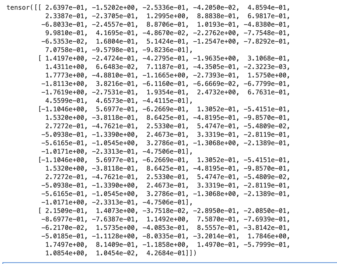
This[5,28] vector shows firing rate of all inputs in each neuron
tensor(0.4859)
e.g. we want to check the score of <S> and a bigram so
(xenc @ W)[26, 0] shows the score of input (<S>) at neuron 0 (output, ‘a’), which later can be calculated to probabilty
Other way to look at this matrix multiplcation:
The one encoded 1 with its specific index, picks an item in weights, different index of weights are showing the weights of the next characters,
Score of bigram (nm) is weight of m at the index that pointed by n
Every input, has 28 outputs because of 28 neurons, which represents the next characters after input, and the score(comes from weights),
We convert scores to probs.
The math works because simply in the matrix multiplication we are multiplying input to output
As you see in the image, still the outputs are not proper for our upcoming nn, (compare loss function, with the current numbers which has negative and positive numbers, so we need to convert them to some numbers positive)
This is where we use exponent simply because it converts any real number into a positive number
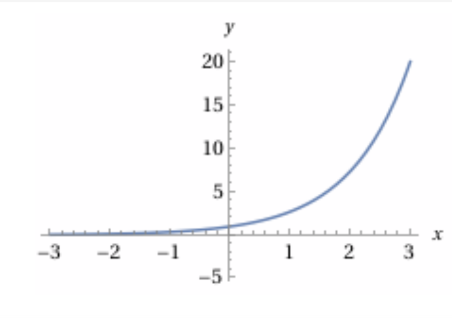
(xenc @ W).exp()
let’s call xenc @ W, logits
just for naming convention, means raw scores before converting into probabilties
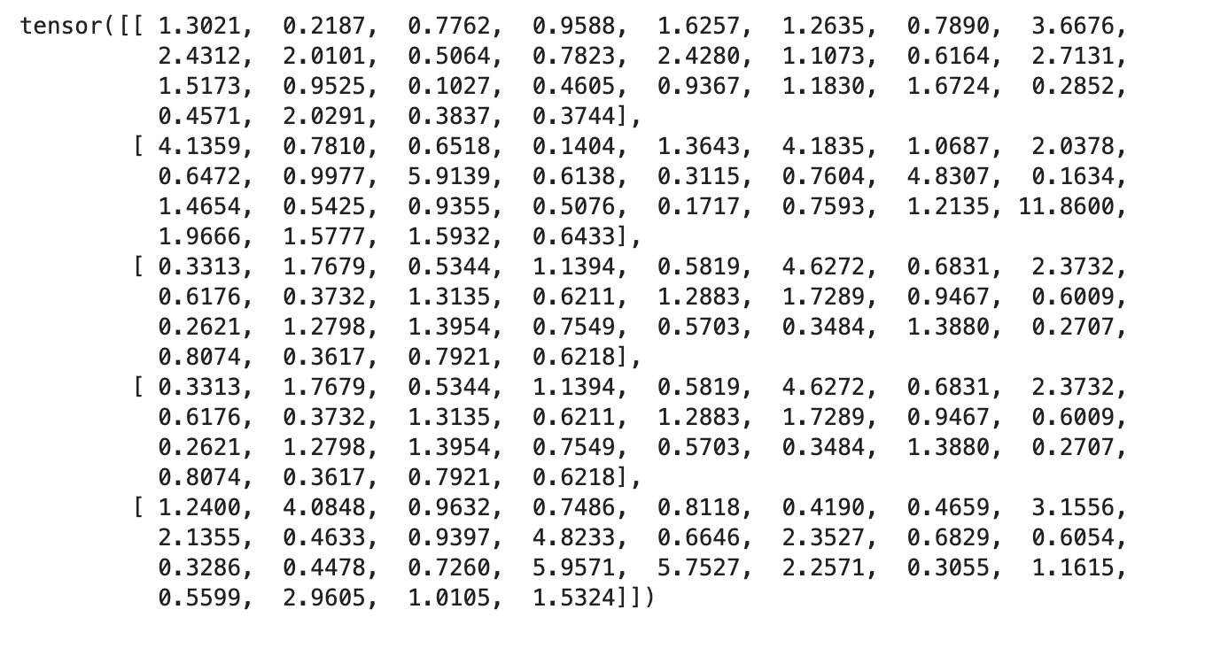
and (xenc @ W).exp(), counts
represents similar behaviour with counts of occouerences of bigrams
Note
logits-> exp()-> normalizing-> prob. dist. This layer also called “Softmax”
and lets create prob. dist. from counts:
probs = counts / counts.sum(1, keepdims=True)
probs
Note: Still we have not added a non inearity such as tanh()
Now that we make the neurons and the weights, and forward pass, we check if we can backpropagate the operations too, which is a necessary step in our nn, and training.
logits = xenc @ W (they are just multiplication and addition)
counts = logits.exp() (we know how to calcualte the local derivative of exp)
probs = counts / counts.sum(1, keepdims=True) (division and sum)
Let’s make an example and wrap up this epoch
allneglogs = torch.zeros(5)
xenc = F.one_hot(xs, num_classes=28).float()
g = torch.Generator().manual_seed(11224234)

W = torch.randn((28, 28), generator=g)
logits = xenc @ W
counts = logits.exp()
probs = counts / counts.sum(1, keepdims=True)

for i in range(5):
    x = xs[i].item()
    y = ys[i].item()
    p = probs[i, y]

    print(itos[x], itos[y])
    print("probability")
    print(p.item())

    neglogp = -(torch.log(p))
    print("neg log")
    print(logp.item())

    allneglogs[i] = neglogp

print("average neg log, also known as loss=")
print(allneglogs.mean().item())
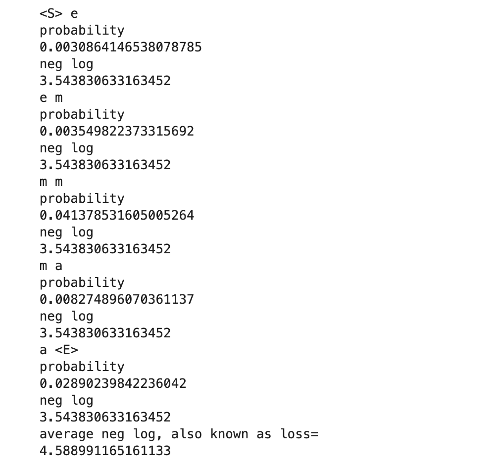
This only calculated the loss for one word.
Later on we can fine tune the Ws by gradient optimization, simiar to what we did in micrograd.